
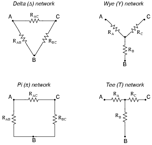
In many circuit applications, we encounter components connected together in one of two ways to form a three-terminal network: the “Delta,” or Δ (also known as the “Pi,” or π) configuration, and the “Y” (also known as the “T”) configuration.
It is possible to calculate the proper values of resistors necessary to form one kind of network (Δ or Y) that behaves identically to the other kind, as analyzed from the terminal connections alone. That is, if we had two separate resistor networks, one Δ and one Y, each with its resistors hidden from view, with nothing but the three terminals (A, B, and C) exposed for testing, the resistors could be sized for the two networks so that there would be no way to electrically determine one network apart from the other. In other words, equivalent Δ and Y networks behave identically.
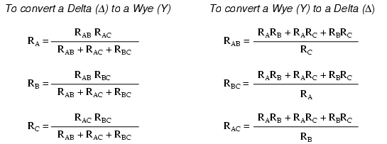
There are several equations used to convert one network to the other:
Δ and Y networks are seen frequently in 3-phase AC power systems (a topic covered in volume II of this book series), but even then they're usually balanced networks (all resistors equal in value) and conversion from one to the other need not involve such complex calculations. When would the average technician ever need to use these equations?
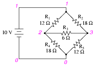
A prime application for Δ-Y conversion is in the solution of unbalanced bridge circuits, such as the one below:
Solution of this circuit with Branch Current or Mesh Current analysis is fairly involved, and neither the Millman nor Superposition Theorems are of any help, since there's only one source of power. We could use Thevenin's or Norton's Theorem, treating R3 as our load, but what fun would that be?
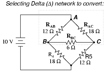
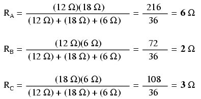
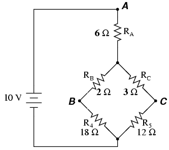
If we were to treat resistors R1, R2, and R3 as being connected in a Δ configuration (Rab, Rac, and Rbc, respectively) and generate an equivalent Y network to replace them, we could turn this bridge circuit into a (simpler) series/parallel combination circuit:
After the Δ-Y conversion . . .
If we perform our calculations correctly, the voltages between points A, B, and C will be the same in the converted circuit as in the original circuit, and we can transfer those values back to the original bridge configuration.
Resistors R4 and R5, of course, remain the same at 18 Ω and 12 Ω, respectively. Analyzing the circuit now as a series/parallel combination, we arrive at the following figures:
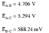
We must use the voltage drops figures from the table above to determine the voltages between points A, B, and C, seeing how the add up (or subtract, as is the case with voltage between points B and C):
Now that we know these voltages, we can transfer them to the same points A, B, and C in the original bridge circuit:
Voltage drops across R4 and R5, of course, are exactly the same as they were in the converted circuit.
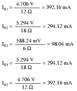
At this point, we could take these voltages and determine resistor currents through the repeated use of Ohm's Law (I=E/R):
A quick simulation with SPICE will serve to verify our work:[spi]
unbalanced bridge circuit
v1 1 0
r1 1 2 12
r2 1 3 18
r3 2 3 6
r4 2 0 18
r5 3 0 12
.dc v1 10 10 1
.print dc v(1,2) v(1,3) v(2,3) v(2,0) v(3,0)
.end
v1            v(1,2)      v(1,3)      v(2,3)      v(2)        v(3)
1.000E+01     4.706E+00   5.294E+00   5.882E-01   5.294E+00   4.706E+00
The voltage figures, as read from left to right, represent voltage drops across the five respective resistors, R1 through R5. I could have shown currents as well, but since that would have required insertion of “dummy” voltage sources in the SPICE netlist, and since we're primarily interested in validating the Δ-Y conversion equations and not Ohm's Law, this will suffice.
* REVIEW:
* “Delta” (Δ) networks are also known as “Pi” (π) networks.
* “Y” networks are also known as “T” networks.
* Δ and Y networks can be converted to their equivalent counterparts with the proper resistance equations. By “equivalent,” I mean that the two networks will be electrically identical as measured from the three terminals (A, B, and C).
* A bridge circuit can be simplified to a series/parallel circuit by converting half of it from a Δ to a Y network. After voltage drops between the original three connection points (A, B, and C) have been solved for, those voltages can be transferred back to the original bridge circuit, across those same equivalent points.
The Maximum Power Transfer Theorem is not so much a means of analysis as it is an aid to system design. Simply stated, the maximum amount of power will be dissipated by a load resistance when that load resistance is equal to the Thevenin/Norton resistance of the network supplying the power. If the load resistance is lower or higher than the Thevenin/Norton resistance of the source network, its dissipated power will be less than maximum.
This is essentially what is aimed for in radio transmitter design , where the antenna or transmission line “impedance” is matched to final power amplifier “impedance” for maximum radio frequency power output. Impedance, the overall opposition to AC and DC current, is very similar to resistance, and must be equal between source and load for the greatest amount of power to be transferred to the load. A load impedance that is too high will result in low power output. A load impedance that is too low will not only result in low power output, but possibly overheating of the amplifier due to the power dissipated in its internal (Thevenin or Norton) impedance.
Taking our Thevenin equivalent example circuit, the Maximum Power Transfer Theorem tells us that the load resistance resulting in greatest power dissipation is equal in value to the Thevenin resistance (in this case, 0.8 Ω):
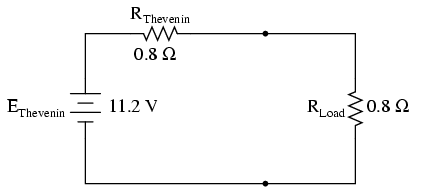
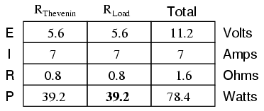
With this value of load resistance, the dissipated power will be 39.2 watts:
If we were to try a lower value for the load resistance (0.5 Ω instead of 0.8 Ω, for example), our power dissipated by the load resistance would decrease:

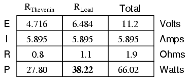
Power dissipation increased for both the Thevenin resistance and the total circuit, but it decreased for the load resistor. Likewise, if we increase the load resistance (1.1 Ω instead of 0.8 Ω, for example), power dissipation will also be less than it was at 0.8 Ω exactly:
If you were designing a circuit for maximum power dissipation at the load resistance, this theorem would be very useful. Having reduced a network down to a Thevenin voltage and resistance (or Norton current and resistance), you simply set the load resistance equal to that Thevenin or Norton equivalent (or vice versa) to ensure maximum power dissipation at the load. Practical applications of this might include radio transmitter final amplifier stage design (seeking to maximize power delivered to the antenna or transmission line), a grid tied inverter loading a solar array, or electric vehicle design (seeking to maximize power delivered to drive motor).
The Maximum Power Transfer Theorem is not: Maximum power transfer does not coincide with maximum efficiency. Application of The Maximum Power Transfer theorem to AC power distribution will not result in maximum or even high efficiency. The goal of high efficiency is more important for AC power distribution, which dictates a relatively low generator impedance compared to load impedance.
Similar to AC power distribution, high fidelity audio amplifiers are designed for a relatively low output impedance and a relatively high speaker load impedance. As a ratio, "output impdance" : "load impedance" is known as damping factor, typically in the range of 100 to 1000. [rar] [dfd]
Maximum power transfer does not coincide with the goal of lowest noise. For example, the low-level radio frequency amplifier between the antenna and a radio receiver is often designed for lowest possible noise. This often requires a mismatch of the amplifier input impedance to the antenna as compared with that dictated by the maximum power transfer theorem.
- REVIEW:
- The Maximum Power Transfer Theorem states that the maximum amount of power will be dissipated by a load resistance if it is equal to the Thevenin or Norton resistance of the network supplying power.
- The Maximum Power Transfer Theorem does not satisfy the goal of maximum efficiency. In many circuit applications, we encounter components connected together in one of two ways to form a three-terminal network: the “Delta,” or Δ (also known as the “Pi,” or π) configuration, and the “Y” (also known as the “T”) configuration.
It is possible to calculate the proper values of resistors necessary to form one kind of network (Δ or Y) that behaves identically to the other kind, as analyzed from the terminal connections alone. That is, if we had two separate resistor networks, one Δ and one Y, each with its resistors hidden from view, with nothing but the three terminals (A, B, and C) exposed for testing, the resistors could be sized for the two networks so that there would be no way to electrically determine one network apart from the other. In other words, equivalent Δ and Y networks behave identically.
There are several equations used to convert one network to the other:
Δ and Y networks are seen frequently in 3-phase AC power systems (a topic covered in volume II of this book series), but even then they're usually balanced networks (all resistors equal in value) and conversion from one to the other need not involve such complex calculations. When would the average technician ever need to use these equations?
A prime application for Δ-Y conversion is in the solution of unbalanced bridge circuits, such as the one below:
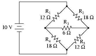
Solution of this circuit with Branch Current or Mesh Current analysis is fairly involved, and neither the Millman nor Superposition Theorems are of any help, since there's only one source of power. We could use Thevenin's or Norton's Theorem, treating R3 as our load, but what fun would that be?
If we were to treat resistors R1, R2, and R3 as being connected in a Δ configuration (Rab, Rac, and Rbc, respectively) and generate an equivalent Y network to replace them, we could turn this bridge circuit into a (simpler) series/parallel combination circuit:
After the Δ-Y conversion . . .
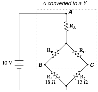
If we perform our calculations correctly, the voltages between points A, B, and C will be the same in the converted circuit as in the original circuit, and we can transfer those values back to the original bridge configuration.
Resistors R4 and R5, of course, remain the same at 18 Ω and 12 Ω, respectively. Analyzing the circuit now as a series/parallel combination, we arrive at the following figures:
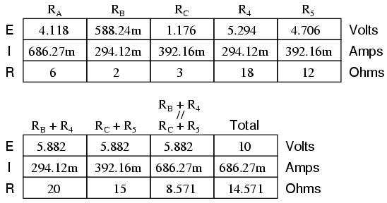
We must use the voltage drops figures from the table above to determine the voltages between points A, B, and C, seeing how the add up (or subtract, as is the case with voltage between points B and C):
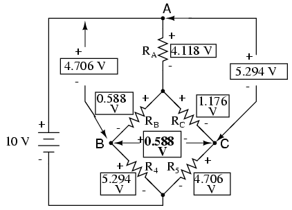
Now that we know these voltages, we can transfer them to the same points A, B, and C in the original bridge circuit:
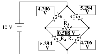
Voltage drops across R4 and R5, of course, are exactly the same as they were in the converted circuit.
At this point, we could take these voltages and determine resistor currents through the repeated use of Ohm's Law (I=E/R):
A quick simulation with SPICE will serve to verify our work:[spi]
unbalanced bridge circuit v1 1 0 r1 1 2 12 r2 1 3 18 r3 2 3 6 r4 2 0 18 r5 3 0 12 .dc v1 10 10 1 .print dc v(1,2) v(1,3) v(2,3) v(2,0) v(3,0) .end
v1 v(1,2) v(1,3) v(2,3) v(2) v(3) 1.000E+01 4.706E+00 5.294E+00 5.882E-01 5.294E+00 4.706E+00
The voltage figures, as read from left to right, represent voltage drops across the five respective resistors, R1 through R5. I could have shown currents as well, but since that would have required insertion of “dummy” voltage sources in the SPICE netlist, and since we're primarily interested in validating the Δ-Y conversion equations and not Ohm's Law, this will suffice.
- REVIEW:
- “Delta” (Δ) networks are also known as “Pi” (π) networks.
- “Y” networks are also known as “T” networks.
- Δ and Y networks can be converted to their equivalent counterparts with the proper resistance equations. By “equivalent,” I mean that the two networks will be electrically identical as measured from the three terminals (A, B, and C).
- A bridge circuit can be simplified to a series/parallel circuit by converting half of it from a Δ to a Y network. After voltage drops between the original three connection points (A, B, and C) have been solved for, those voltages can be transferred back to the original bridge circuit, across those same equivalent points.


No comments:
Post a Comment